Fluid Dynamics

With the help of the fluid dynamics simulation tools of Realsoft 3D, you can easily animate various fluid or air flow related phenomena:

• A falling object accelerating slowly towards the terminal velocity
• A fan that blows a bunch of objects away
• Aerodynamic properties of a moving dart turn its peak forward

Terminal velocity of falling objects

The first example demonstrates how atmosphere resists rapid motions. Because of this, the velocity of a falling object does not increase forever but approaches the so called terminal velocity.

Tutorial level: Medium

Tutorial example: 'tutorprojects/simulation/falling_objects'

1. Create two analytic spheres, one big and one small.

2. Activate the Gravity tool from the 'Simulation' tab of the toolbar. Draw a vertical line showing the direction of gravity on a view window.

3. Select the two spheres. Open the property window, go to the 'Sim' tab and set 'Gravity' = 'Affected' for the spheres.

4. Select the parent level and turn 'Simulation' on from the tool control bar.

5. Set the frame count to 500 and play the animation.

The natural earth-like gravity accelerates the spheres very rapidly and they disappear from the view window. Stop the playback after about 50 frames. If you look at the 'Velocity' value of the spheres from the property window's 'Phys' tab, you can see that both spheres have exactly the same velocity (which is already quite high, over 20 m/s = 72 km/h). The velocity does not depend on the size of spheres.

6. Rewind the animation.

7. Select the Fan tool from the 'Simulation' tool tab. Draw a fan object with three mouse clicks on a view window: 1. fan position, 2. fan direction, 3. fan radius. The size and orientation of fan is not important this time.

The fan tool selected

8. Go to the 'Phys' tab of the fan's property window. Set 'Fluid Velocity' of the fan to zero (default value is 10 m/s). The reason is that we do not want any wind blowing in this simulation. The fan only adds a non-flowing atmosphere which resists motions.

9. Increase the 'Density' value (it is also in the 'Phys' tab) of the fan from 1.0 to 10.0 kg/cubic meters. The denser the media, the better it resists motions.

10. Select the two spheres. Switch to the 'Sim' tab and set 'Fluid Dynamics' = 'Affected'.

Turn 'Fluid Dynamics' on

11. Play the animation. The spheres start falling again. Now the smaller sphere falls faster. The spheres have an equal default mass of 1 kg. However, the small sphere has a smaller area causing air friction, and therefore it can fall quicker. This is a correct result - a small stone falls quickly, but if you put it inside a balloon it falls slowly.

You may stop the playback again after 50 frames. The property window shows that velocities are now smaller, probably less than 20 m/s. Rewind the animation.

12. As a final step, select the two spheres and decrease the 'Mass' value to 0.1 kg using the 'Phys' tab of the property window. Play the animation again. Now the air resistance is quite significant because of the low weight of the spheres. Both reach their terminal velocity quickly during the first 50 frames. The terminal velocity of the bigger sphere is quite low, less than 5 meters per second.

A funny fan

You may have already noticed that the 'Fluid Dynamics' gadget includes the same list of alternatives as the 'Collision Detection' and force fields: Cause - Affected - Both - Inactive. This means that any object can generate the fluid medium and a flow to it. However, there is one special purpose object available for this purpose, namely the fan object.

A fluid flow generated by an ordinary object, for example a NURBS line, is constant everywhere. A fan can generate non-uniform and turbulent flows. The following example demonstrates this.

Tutorial level: Medium

Example project: 'tutorprojects/simulation/fan'

1. Create a 'creator' object by using the select window's popup menu 'New/Creator'.

2. Create a small sphere to the left edge of the view window. Open the property window, go to the 'Sim' tab and define 'Fluid Dynamics' = 'Affected'. Even a strong wind cannot move small round objects that weight 1 kilogram (probably made of lead). Therefore, switch to the 'Phys' tab and change 'Mass' to '0.001' (= one gram). Then drop the sphere into the sub hierarchy of the creator object.

3. Activate the Fan tool from the 'Simulation ' tool tab. Draw a fan in the middle of the view window. The third mouse click defines the fan diameter; it should be about 10-20 % of the view window's width (see the image below).

The fan in action

4. Go to the 'Phys' tab of the fan's property window. Set the 'Spin' value of the fan to '4 0 0'. This will make the fan rotate. Increase the 'Fluid Velocity' value to 200 m/s, and 'Density' to '10'. This is a truly powerful fan, which can move the spheres easily!

5. Switch to the 'Spec' tab containing the fan specific options. First set 'Turbulence' to 0.3 - this will produce slightly turbulent airflow, like all real world fans do.

Properties of the fan

6. Both 'Radial falloff' and 'Axis falloff' gadgets are 'Constant' by default. This means that the fan is really strong - it creates a wind that blows through the whole universe. Change both 'Radial falloff' and 'Axis falloff' to 'Linear'. Now the airflow will drop to zero outside the radius of the fan, and get weaker as the distance along the fan axis grows (flow is inversely proportional to the distance). The third alternative 'Quadric' also produces a local airflow, but the falloff is more rapid.

7. Close the property window. Turn on 'Simulation' of the parent level and play the animation.

A flying dart

So far, we have used simple symmetric objects for testing fluid dynamics. We have already seen some examples of force fields that spin objects having a suitable sub structure:

• A pendulum in a gravity field
• A compass needle in a electro magnetic force field

By using compound objects consisting of several parts, the same kind of fluid effects can be achieved. The fluid simulation system examines sub hierarchies of objects and each sub component generates its own contribution to the total result. If the mass/area distribution is not symmetric, the result force rotates the object.

The next example, a flying dart, shows this kind of situation. The dart is thrown and it starts falling in a gravity field. The shape of the dart is such that airflow automatically turns the sharp peak of the dart to point to the direction where the dart is moving.

Tutorial level: Medium

Example project: 'tutorprojects/simulation/dart'

1. Model a dart using suitable components. For example, model the two wings at the tail by using two spheres, which are stretched flat in one dimension. The body of the dart can be a cylinder with two spheres at the ends. An analytic cone forms the peak. Enclose all the components in a hierarchy level called 'dart'.

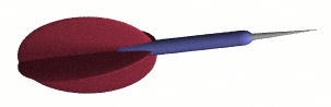
A dart

2. Place the dart to the left edge of the view. Direct it to the right and slightly upwards, which is a good starting position for the dart.

3. Go to the 'Simulation' tab of the toolbar. Make sure the dart is selected and start the Velocity tool. Draw a velocity line halfway through the view, to the direction of the dart. The line shows how you 'throw' the dart.

4. Click the Gravity tool of the 'Simulation' tab and draw a gravity line pointing downwards (the length is not important, only the direction).

5. Activate the Fan tool and draw a fan in a view window. Then select the parent level of created objects (root) and turn 'Simulation' on from the tool control bar.

 
The components of the dart simulation

All the required components of the simulation are now included, but we have to adjust some simulation and physical properties. Let's start from the dart itself: 

 6. Select the dart and open the property window. Go to the 'Sim' tab. Set 'Gravity' = 'Affected' and 'Fluid Dynamics' = 'Affected'.

 Now the simulation already works, but the default properties are quite poor. For example, the default weight of the small dart is several kilograms!

7. Go to the 'Phys' tab. Select the tail components of the dart and set 'Mass' field to '0.001' (one gram). Remember you can set the number of decimals in the Options/Window/Metrics tab from the main menu. Then select the body components and set their mass to '0.003' (three grams). Finally, select the peak and the front part of the body, and set the mass to '0.01' kilograms. If you select the 'dart' level, you can check the total mass, which is automatically computed form the components: it is now '0.02' - '0.03' i.e. some tens of grams. This is quite a realistic value. Note that the center of gravity is in the front part of the dart. If you have tried playing with 'real' darts, you know that they are designed this way.

Now the dart works better. However, in earth's gravity a dart falls very rapidly and hence it must also fly very rapidly to reach its goal. In order to see properly how the dart flies, let's define a 'slow motion' simulation setup.

8. Select the 'Gravity' object from the hierarchy. Go to the 'Spec' tab and decrease the 'Strength' from 9.82 (earth gravity) to 0.1. Now the dart will fall more slowly.

9. Select the 'Fan' and go to the 'Phys' tab. Set 'Fluid Velocity' to zero (no wind).

10. A normal atmosphere does not affect the 'slow motion' dart much. Therefore, increase the 'Density' value from 1 to 10.

You can now close the property window. Set the fame count to 150-250 frames, turn on Simulation for the Root level and play the animation to see the result.

Note: The dart will turn easier if you decrease the default 'Inertia' value. The program estimates the default inertia from the mass and object dimensions. The estimated value can be inaccurate. A real dart's mass is heavily concentrated in the front part, which is made of heavy metal, whereas the plastic tail does not weight much. Therefore, the correct inertia value is quite low. For example, divide all the three default inertia components by five.